Tutorial 4: CostGrow and Model Comparison

This tutorial builds on Tutorial 2 by running the same sample data through both the built-in CostGrow_Terrain model and the downloaded ResUNet_16x_DEM model.

By the end, you will have:

• a CostGrow output raster

• a ResUNet output raster

• a comparison raster storing CostGrow - ResUNet

• a side-by-side plot of the two model outputs

Before you start

This tutorial requires the extended install because CostGrow_Terrain depends on PCRaster.

• CLI (pipx): use the extended environment from Command line (CLI) - Extended.

• Local notebook (Jupyter): use the extended environment from Local notebook (Jupyter) - Extended.

• Hosted notebook (Colab): not recommended for this tutorial because the extended stack is heavier and less reliable.

Install additional packages

# %pip install -q matplotlib rasterio

Prove the install

Let’s check the versions now:

import matplotlib
import rasterio

print(f"matplotlib=={matplotlib.__version__}")
print(f"rasterio=={rasterio.__version__}")

matplotlib==3.10.8
rasterio==1.5.0

!floodsr --version

Imports

from pathlib import Path
from urllib.request import urlretrieve

import matplotlib.pyplot as plt
import numpy as np
import rasterio

Download the same test data as Tutorial 2

We reuse the small sample rasters from the earlier tutorials so the comparison stays quick to run and easy to inspect.

urlretrieve(
    "https://github.com/cefect/floodsr/releases/download/v0.0.3/hires002_dem.tif",
    "hires002_dem.tif",
)
urlretrieve(
    "https://github.com/cefect/floodsr/releases/download/v0.0.3/lowres032.tif",
    "lowres032.tif",
)

('lowres032.tif', <http.client.HTTPMessage at 0x7374613018e0>)

Resolve the input paths

lowres_fp = Path("lowres032.tif").resolve()
dem_fp = Path("hires002_dem.tif").resolve()
assert lowres_fp.is_file(), f"missing low-res raster\n    {lowres_fp}"
assert dem_fp.is_file(), f"missing DEM raster\n    {dem_fp}"

costgrow_fp = Path("lowres032_costgrow_sr.tif").resolve()
resunet_fp = Path("lowres032_resunet_sr.tif").resolve()
comparison_fp = Path("lowres032_costgrow_minus_resunet.tif").resolve()

Fetch ResUNet weights

CostGrow_Terrain is built in, so it does not need a weights download. ResUNet_16x_DEM does, so we fetch it once here before running the comparison.

!floodsr models fetch --no-progress ResUNet_16x_DEM

version=ResUNet_16x_DEM stored=/tmp/.cache/floodsr/ResUNet_16x_DEM/model_infer.onnx retrieved_from=cache

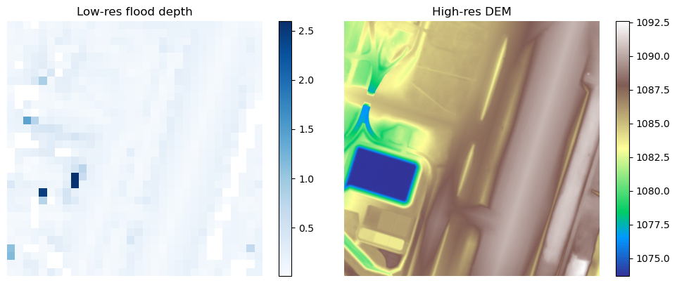
Plot the tutorial inputs

def read_raster_band_1(fp):
    """Read band 1 as float and promote masked nodata pixels to NaN."""
    assert Path(fp).is_file(), f"missing raster\n    {fp}"
    with rasterio.open(fp) as src:
        return src.read(1, masked=True).astype(float).filled(np.nan)


def write_float_raster_like(reference_fp, out_fp, arr):
    """Write one float32 raster using the profile from a reference raster."""
    with rasterio.open(reference_fp) as src:
        profile = src.profile.copy()
    profile.update(dtype="float32", count=1, nodata=np.nan)
    with rasterio.open(out_fp, "w", **profile) as dst:
        dst.write(arr.astype("float32"), 1)

lowres_arr = read_raster_band_1(lowres_fp)
dem_arr = read_raster_band_1(dem_fp)

fig, axes = plt.subplots(1, 2, figsize=(10, 4))

im0 = axes[0].imshow(np.where(lowres_arr > 0, lowres_arr, np.nan), cmap="Blues")
axes[0].set_title("Low-res flood depth")
fig.colorbar(im0, ax=axes[0])
axes[0].set_axis_off()

im1 = axes[1].imshow(dem_arr, cmap="terrain")
axes[1].set_title("High-res DEM")
fig.colorbar(im1, ax=axes[1])
axes[1].set_axis_off()
fig.tight_layout()

Run CostGrow

Now run tohr with the built-in CostGrow_Terrain model. We set --window-method hard explicitly so the tutorial reflects the current large-raster-safe CostGrow path.

!floodsr -q tohr --in lowres032.tif --dem hires002_dem.tif --model-version CostGrow_Terrain --window-method hard --tile-overlap 0 --out lowres032_costgrow_sr.tif

Run the ResUNet baseline

Next run the learned ResUNet_16x_DEM model on the same inputs so we can compare the two outputs directly.

!floodsr -q tohr --in lowres032.tif --dem hires002_dem.tif --model-version ResUNet_16x_DEM --out lowres032_resunet_sr.tif

Write a comparison raster

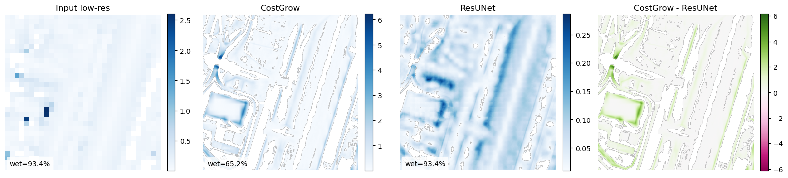
For a quick numeric comparison, we save a raster of CostGrow - ResUNet on the same grid as the model outputs. Positive values indicate deeper predictions from CostGrow, and negative values indicate deeper predictions from ResUNet.

costgrow_arr = read_raster_band_1(costgrow_fp)
resunet_arr = read_raster_band_1(resunet_fp)
comparison_arr = costgrow_arr - resunet_arr
write_float_raster_like(costgrow_fp, comparison_fp, comparison_arr)
comparison_arr

Plot the results side by side

The first three panels compare the input and the two high-resolution outputs. The fourth panel shows the signed difference raster so you can quickly spot where the model outputs diverge.

fig, axes = plt.subplots(1, 4, figsize=(16, 4))
plot_l = [
    (axes[0], np.where(lowres_arr > 0, lowres_arr, np.nan), "Input low-res", "Blues"),
    (axes[1], np.where(costgrow_arr > 0, costgrow_arr, np.nan), "CostGrow", "Blues"),
    (axes[2], np.where(resunet_arr > 0, resunet_arr, np.nan), "ResUNet", "Blues"),
]
for ax, arr, title, cmap in plot_l:
    wet_pct = 100.0 * float(np.count_nonzero(np.nan_to_num(arr, nan=0.0) > 0.0)) / float(arr.size)
    im = ax.imshow(arr, cmap=cmap)
    ax.set_title(title)
    ax.axis("off")
    ax.text(0.03, 0.03, f"wet={wet_pct:.1f}%", transform=ax.transAxes, color="black", fontsize=10, bbox={"facecolor": "white", "alpha": 0.8, "edgecolor": "none"})
    fig.colorbar(im, ax=ax, fraction=0.046, pad=0.04)

delta_vmax = float(np.nanmax(np.abs(comparison_arr)))
if not np.isfinite(delta_vmax) or delta_vmax == 0.0:
    delta_vmax = 1.0
im_delta = axes[3].imshow(comparison_arr, cmap="PiYG", vmin=-delta_vmax, vmax=delta_vmax)
axes[3].set_title("CostGrow - ResUNet")
axes[3].axis("off")
fig.colorbar(im_delta, ax=axes[3], fraction=0.046, pad=0.04)
fig.tight_layout()