Tutorial 2: Plotting and Advanced Options#

This tutorial expands on Tutorial 1 with visualization and demonstrating the behavior of some key CLI options.

This tutorial assumes you have floodsr installed per Tutorial 1 and are comfortable with simple python notebooks. If you’ve never used a Jupyter notebook before, we recommend checking out the Intro Notebooks from Project Jupyter to get familiar with the interface and basic features.

There are three common ways to run this tutorial (i.e., execution contexts):

command line (CLI): proceed by copy/pasting the below commands from your web-browser into your terminal. NOTE for most terminals you’ll need to remove the prefix ! from each command.
local notebook (Jupyter): Use the button to save this notebook as an .ipynb file to your local machine (may need to click save as) and open it with your local Jupyter kernel. see Local notebook (Jupyter) for details.
hosted notebook (Colab): Use the button to open this tutorial on Google Colab.

Install additional packages#

For this tutorial, we need the additional python packages matplotlib and rasterio. Like the install of floodsr shown in Tutorial 1, obtaining and implementing these packages depends on your execution context:

The appropriate installation steps depend on your execution context, which is described in detail in Basic Install. Here are the basic steps for each:

command line (CLI): first, ensure pipx is installed and on PATH, then run pipx install floodsr. see Command line (CLI) for more details.
local notebook (Jupyter): same as above. then either follow the additional steps in Local notebook (Jupyter) to properly set up your environment, or be lazy and uncomment the below Jupyter cell and run.
hosted notebook (Colab): uncomment the below colab cell and run. see Hosted notebook (Colab) for details.

# %pip install -q matplotlib rasterio

Prove the install#

Let’s check the versions now:

import matplotlib
import rasterio

print(f"matplotlib=={matplotlib.__version__}")
print(f"rasterio=={rasterio.__version__}")

matplotlib==3.10.8
rasterio==1.5.0

!floodsr --version

floodsr 0.1.2.dev37

Imports#

Here we import our tools and create a small helper function for reading raster data

from pathlib import Path
from urllib.request import urlretrieve

import matplotlib.pyplot as plt
import numpy as np
from rasterio.warp import Resampling, calculate_default_transform, reproject

Download the same test data as Tutorial 1#

If you already downloaded these files while working through Tutorial 1, you can skip this.

urlretrieve(
    "https://github.com/cefect/floodsr/releases/download/v0.0.3/hires002_dem.tif",
    "hires002_dem.tif",
)
urlretrieve(
    "https://github.com/cefect/floodsr/releases/download/v0.0.3/lowres032.tif",
    "lowres032.tif",
)

('lowres032.tif', <http.client.HTTPMessage at 0x76aab7621b50>)

Here we map the downloaded paths to variables for convenience (and check that they exist)

lowres_fp = Path("lowres032.tif").resolve()
dem_fp = Path("hires002_dem.tif").resolve()
assert lowres_fp.is_file(), f"missing low-res raster\n    {lowres_fp}"
assert dem_fp.is_file(), f"missing DEM raster\n    {dem_fp}"

Fetch model weights#

You can skip this if you just ran Tutorial 1, but re-fetching is best-practice and harmless (if the file already exist, it won’t be re-downloaded).

!floodsr models fetch --no-progress ResUNet_16x_DEM

version=ResUNet_16x_DEM stored=/tmp/.cache/floodsr/ResUNet_16x_DEM/model_infer.onnx retrieved_from=cache

Plot the tutorial inputs#

First, lets define a simple function to help us load raster data into the plots

def read_raster_band_1(fp):
    """Read band 1 as float and promote masked nodata pixels to NaN."""
    assert Path(fp).is_file(), f"missing raster\n    {fp}"
    with rasterio.open(fp) as src:
        return src.read(1, masked=True).astype(float).filled(np.nan)

Now we create a simple plot of the low-res inputs and the high-res DEM we downloaded.

# Read both inputs with masked nodata promoted to NaN for plotting.
lowres_arr = read_raster_band_1(lowres_fp)
dem_arr = read_raster_band_1(dem_fp)

# setup the figure
fig, axes = plt.subplots(1, 2, figsize=(10, 4))

# add the flood raster to the left with a blue colormap, masking nodata values
im0 = axes[0].imshow(np.where(lowres_arr > 0, lowres_arr, np.nan), cmap="Blues")
axes[0].set_title("Low-res flood depth")
fig.colorbar(im0, ax=axes[0])
axes[0].set_axis_off()

# add the DEM raster to the right with a terrain colormap
im1 = axes[1].imshow(dem_arr, cmap="terrain")
axes[1].set_title("High-res DEM")
fig.colorbar(im1, ax=axes[1])
axes[1].set_axis_off()

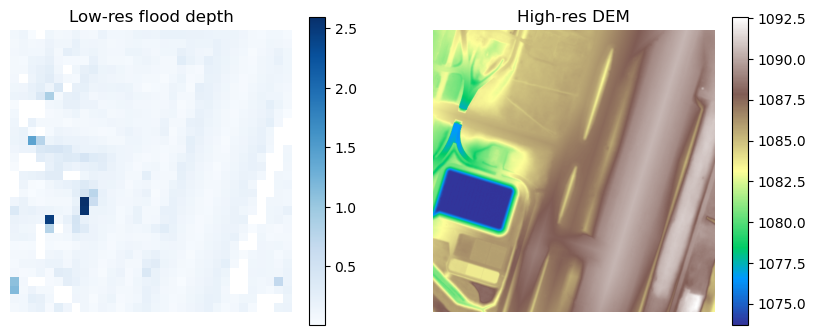
../_images/02284b62618fe36fbdab010826d79375868643a60d179444b74f05e66387b2a0.png

this shows the not-so-great coarse pluvial flood raster at 32m

Plot the Tutorial 1 outputs#

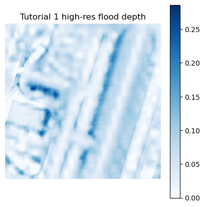
Now let’s rebuild the high-resolution flood depth raster using the same command as Tutorial 1, and plot the result.

# Run the default threshold first so we have a baseline for comparison.
!floodsr -q tohr --in lowres032.tif --dem hires002_dem.tif --out lowres032_default_sr.tif

feather pass:   0%|                                   | 0/1 [00:00<?, ?window/s]

feather pass: 100%|███████████████████████████| 1/1 [00:00<00:00, 19.29window/s]

final write pass:   0%|                              | 0/128 [00:00<?, ?block/s]
final write pass: 100%|█████████████████| 128/128 [00:00<00:00, 10387.77block/s]
/home/cefect/LS/10_IO/2407_FHIMP/tmp/floodsr-tutorial_2-2bmo3t/run/lowres032_default_sr.tif

And a quick plot:

arr = read_raster_band_1("lowres032_default_sr.tif")

fig, ax = plt.subplots(figsize=(5, 5))
im = ax.imshow(arr, cmap="Blues")
ax.set_title("Tutorial 1 high-res flood depth")
fig.colorbar(im, ax=ax)
ax.set_axis_off()

../_images/b4440ca1557d0dc61162b79996c44a21b56d7e384b1c7e4e2376489e587ac171.png

CRS policies#

Here we demonstrate the behaviour of floodsr when the input rasters have mismatched CRS information, and how to use the --crs-policy option to control this behaviour.

Probe the CRS of both rasters#

A coordinate reference system (CRS) tells raster software how pixel locations map onto real-world coordinates. Ideally, your data is all on some obvious, common CRS (e.g., NAD83(CSRS) / Canada Atlas Lambert aka EPSG:3979), but in practice you may encounter rasters with missing or mismatched CRS information; and we need to tell floodsr how to handle these cases.

Before we trigger a CRS mismatch on purpose, let’s inspect the CRS metadata on the original rasters.

with rasterio.open(lowres_fp) as src:
    print(f"{lowres_fp.name}: crs={src.crs} shape={src.shape} res={src.res}")

with rasterio.open(dem_fp) as src:
    print(f"{dem_fp.name}: crs={src.crs} shape={src.shape} res={src.res}")

lowres032.tif: crs=EPSG:3979 shape=(32, 32) res=(32.0, 32.0)
hires002_dem.tif: crs=EPSG:3979 shape=(512, 512) res=(2.0, 2.0)

Here we see that the CRS of both rasters are identical.

Nice for simple test data, but not so interesting for demonstrating how floodsr handles CRS mismatch. Let’s mix it up.

Create a CRS mismatch#

To demonstrate --crs-policy, we reproject the low-resolution raster to 3978 using rasterio CLI and save it as a new GeoTIFF.

!rio warp lowres032.tif lowres032_epsg3978.tif --dst-crs EPSG:3978 --resampling nearest --co TILED=YES

Run `tohr` with the mismatched CRS#

This command should fail because the low-resolution raster and the DEM no longer share the same CRS and we haven’t told floodsr how to handle this mismatch yet, so it assumes --crs-policy strict by default.

!floodsr tohr --in lowres032_epsg3978.tif --dem hires002_dem.tif

INFO:floodsr.cli:loaded ORT model 'model_infer.onnx' with providers=['CPUExecutionProvider'] and scale=16
INFO:floodsr.cli:tohr path selection
  requested_window_method=feather
  dem_float32_bytes=1,048,576
  windowed_io_threshold_bytes=33,554,432
  selected_platform_materialization=simple
ERROR:floodsr.cli:CRS mismatch under --crs-policy strict
    depth=EPSG:3978
    dem=EPSG:3979

What `--crs-policy` does#

--crs-policy controls how floodsr handles CRS mismatches between the low-resolution depth raster and the DEM. This is necessary because tohr needs the rasters to line up on a common projected grid before preprocessing and inference can proceed, and there is not an obvious “right answer” for which CRS to use when they don’t match.

For this example we use --crs-policy=use-dem, which tells floodsr to treat the DEM CRS as the target CRS and reproject the low-resolution depth raster to match it. We could have chosen --crs-policy=use-lores which would treat the low-resolution raster CRS as the target and reproject the DEM to match it.

!floodsr tohr --in lowres032_epsg3978.tif --dem hires002_dem.tif --crs-policy=use-dem --out lowres032_epsg3978_use_dem_sr.tif

INFO:floodsr.cli:loaded ORT model 'model_infer.onnx' with providers=['CPUExecutionProvider'] and scale=16

INFO:floodsr.cli:tohr path selection
  requested_window_method=feather
  dem_float32_bytes=1,048,576
  windowed_io_threshold_bytes=33,554,432
  selected_platform_materialization=simple
WARNING:floodsr.cli:CRS mismatch; applying --crs-policy=use-dem to resolve a canonical target grid
    depth=EPSG:3978
    dem=EPSG:3979
    target=EPSG:3979

INFO:floodsr.cli:starting tohr inference with model_version=ResUNet_16x_DEM
model
    /tmp/.cache/floodsr/ResUNet_16x_DEM/model_infer.onnx
platform_depth_lr
    /home/cefect/LS/10_IO/2407_FHIMP/tmp/floodsr-tutorial_2-2bmo3t/tmp/floodsr-platform-prep-t3m1rgp1/lowres032_epsg3978_platform_depth.tif
platform_dem_hr
    /home/cefect/LS/10_IO/2407_FHIMP/tmp/floodsr-tutorial_2-2bmo3t/tmp/floodsr-platform-prep-t3m1rgp1/hires002_dem_platform_dem.tif
output
    /home/cefect/LS/10_IO/2407_FHIMP/tmp/floodsr-tutorial_2-2bmo3t/run/lowres032_epsg3978_use_dem_sr.tif
INFO:floodsr.cli:platform-preprocessed inputs
  depth_lr shape=(32, 32) res=(32.0, 32.0) m/pix
  dem_hr shape=(512, 512) res=(2.0, 2.0) m/pix
INFO:floodsr.cli:model preprocessing complete
INFO:floodsr.cli:tohr execution path
  window_method=feather
  execution_path=simple
  model_space_shape=(512, 512)
  raw_output_shape=(512, 512)
INFO:floodsr.cli:prepared inputs summary:
  aligned depth_lr shape=(32, 32) res=(32.0, 32.0) m/pix
  aligned dem_hr shape=(512, 512) res=(2.0, 2.0) m/pix
  max_depth=5.0
  dem_pct_clip=95.0
INFO:floodsr.cli:window config
  method=feather
  overlap_lr=8
  overlap_hr=128
  tile_size_lr=32
  tile_size_hr=512
INFO:floodsr.cli:running feather tiling over 1x1 grid
  stride_hr=384
  overlap_hr=128

feather pass:   0%|                                   | 0/1 [00:00<?, ?window/s]

feather pass: 100%|███████████████████████████| 1/1 [00:00<00:00, 17.85window/s]

final write pass:   0%|                              | 0/128 [00:00<?, ?block/s]
final write pass: 100%|██████████████████| 128/128 [00:00<00:00, 7163.25block/s]
INFO:floodsr.cli:finished tohr inference in 0.093s; wrote 1,116,817 bytes to
    /home/cefect/LS/10_IO/2407_FHIMP/tmp/floodsr-tutorial_2-2bmo3t/run/lowres032_epsg3978_use_dem_sr.tif
/home/cefect/LS/10_IO/2407_FHIMP/tmp/floodsr-tutorial_2-2bmo3t/run/lowres032_epsg3978_use_dem_sr.tif

# Check that the expected output raster exists.
assert Path("lowres032_epsg3978_use_dem_sr.tif").is_file(), "missing output raster\n    lowres032_epsg3978_use_dem_sr.tif"

Plot the CRS-policy result#

Let’s compare the --crs-policy=use-dem result against the baseline output from the original matching-CRS run.

default_fp = Path("lowres032_default_sr.tif").resolve()
use_dem_fp = Path("lowres032_epsg3978_use_dem_sr.tif").resolve()
default_arr = read_raster_band_1(default_fp)
use_dem_arr = read_raster_band_1(use_dem_fp)

fig, axes = plt.subplots(1, 2, figsize=(9, 4))
plot_l = [
    (axes[0], np.where(default_arr > 0, default_arr, np.nan), "Baseline (`lowres032_default_sr.tif`)"),
    (axes[1], np.where(use_dem_arr > 0, use_dem_arr, np.nan), "`--crs-policy=use-dem`")
]
for ax, arr, title in plot_l:
    wet_pct = 100.0 * float(np.count_nonzero(np.nan_to_num(arr, nan=0.0) > 0.0)) / float(arr.size)
    ax.imshow(arr, cmap="Blues")
    ax.set_title(title)
    ax.axis("off")
    ax.text(0.03, 0.03, f"wet={wet_pct:.1f}%", transform=ax.transAxes, color="black", fontsize=10, bbox={"facecolor": "white", "alpha": 0.8, "edgecolor": "none"})
fig.tight_layout()

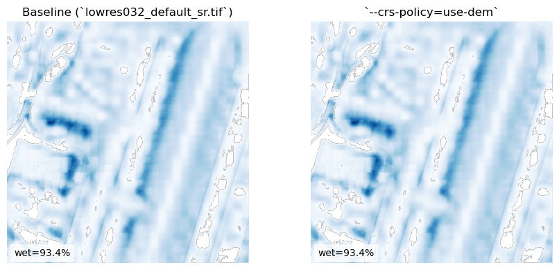
../_images/07316f8dd76e0c24afa5723ac94bfccc086d91fbf515da3c665f6ad4276e2ca2.png

Looks the same to me! as expected…

Check out the FAQ for more discussion on CRS policies.

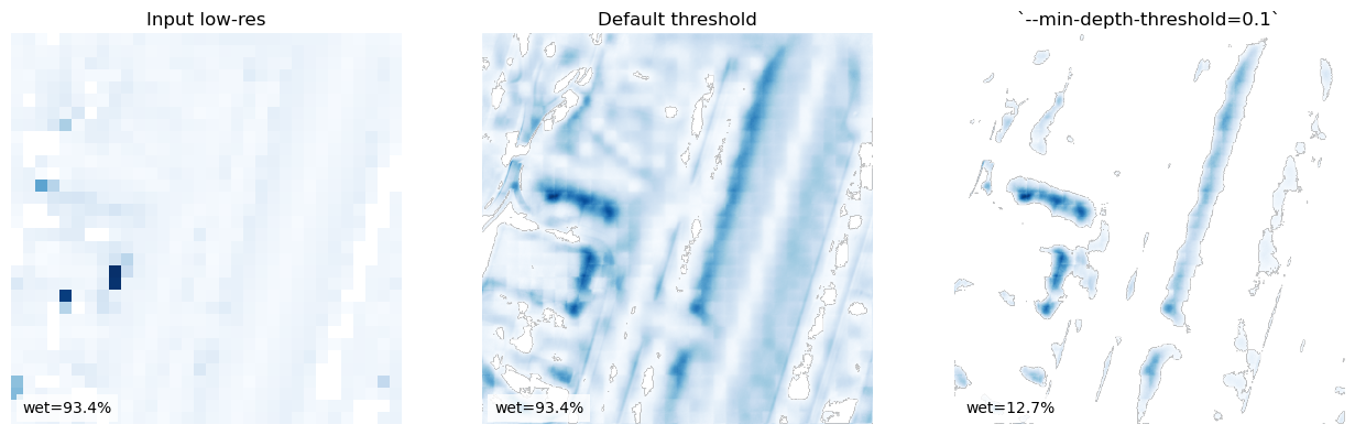
Minimum depth threshold#

Now lets explore the argument --min-depth-threshold, which sets the minimum predicted depth retained in the output raster. Values below the threshold are written as 0.0.

This is useful because very small positive predictions can be noisy or physically improbable, making it an important parameter for tuning the result.

We already ran tohr with the default --min-depth-threshold (0.01) above as a baseline, so now let’s run it again with a higher threshold of 0.1 for comparison.

you’ll noticed we used the -q or --quiet flag to suppress the usual CLI output here.

Now let’s run tohr with a higher --min-depth-threshold of 0.1.

!floodsr tohr --in lowres032.tif --dem hires002_dem.tif --min-depth-threshold=0.1 --out lowres032_min_depth_01_sr.tif

INFO:floodsr.cli:loaded ORT model 'model_infer.onnx' with providers=['CPUExecutionProvider'] and scale=16
INFO:floodsr.cli:tohr path selection
  requested_window_method=feather
  dem_float32_bytes=1,048,576
  windowed_io_threshold_bytes=33,554,432
  selected_platform_materialization=simple

INFO:floodsr.cli:starting tohr inference with model_version=ResUNet_16x_DEM
model
    /tmp/.cache/floodsr/ResUNet_16x_DEM/model_infer.onnx
platform_depth_lr
    /home/cefect/LS/10_IO/2407_FHIMP/tmp/floodsr-tutorial_2-2bmo3t/tmp/floodsr-platform-prep-x7k3jaom/lowres032_platform_depth.tif
platform_dem_hr
    /home/cefect/LS/10_IO/2407_FHIMP/tmp/floodsr-tutorial_2-2bmo3t/tmp/floodsr-platform-prep-x7k3jaom/hires002_dem_platform_dem.tif
output
    /home/cefect/LS/10_IO/2407_FHIMP/tmp/floodsr-tutorial_2-2bmo3t/run/lowres032_min_depth_01_sr.tif
INFO:floodsr.cli:platform-preprocessed inputs
  depth_lr shape=(32, 32) res=(32.0, 32.0) m/pix
  dem_hr shape=(512, 512) res=(2.0, 2.0) m/pix
INFO:floodsr.cli:model preprocessing complete
INFO:floodsr.cli:tohr execution path
  window_method=feather
  execution_path=simple
  model_space_shape=(512, 512)
  raw_output_shape=(512, 512)
INFO:floodsr.cli:prepared inputs summary:
  aligned depth_lr shape=(32, 32) res=(32.0, 32.0) m/pix
  aligned dem_hr shape=(512, 512) res=(2.0, 2.0) m/pix
  max_depth=5.0
  dem_pct_clip=95.0
INFO:floodsr.cli:window config
  method=feather
  overlap_lr=8
  overlap_hr=128
  tile_size_lr=32
  tile_size_hr=512
INFO:floodsr.cli:running feather tiling over 1x1 grid
  stride_hr=384
  overlap_hr=128

feather pass:   0%|                                   | 0/1 [00:00<?, ?window/s]

feather pass: 100%|███████████████████████████| 1/1 [00:00<00:00, 15.60window/s]

final write pass:   0%|                              | 0/128 [00:00<?, ?block/s]
final write pass: 100%|█████████████████| 128/128 [00:00<00:00, 20467.82block/s]
INFO:floodsr.cli:finished tohr inference in 0.089s; wrote 160,772 bytes to
    /home/cefect/LS/10_IO/2407_FHIMP/tmp/floodsr-tutorial_2-2bmo3t/run/lowres032_min_depth_01_sr.tif
/home/cefect/LS/10_IO/2407_FHIMP/tmp/floodsr-tutorial_2-2bmo3t/run/lowres032_min_depth_01_sr.tif

Plot#

# Resolve the two outputs we want to compare.
default_fp = Path("lowres032_default_sr.tif").resolve()
threshold_fp = Path("lowres032_min_depth_01_sr.tif").resolve()
default_arr = read_raster_band_1(default_fp)
threshold_arr = read_raster_band_1(threshold_fp)

# Plot the input and both thresholded outputs side by side.
fig, axes = plt.subplots(1, 3, figsize=(13, 4))
plot_l = [
    (axes[0], np.where(lowres_arr > 0, lowres_arr, np.nan), "Input low-res"),
    (axes[1], np.where(default_arr > 0, default_arr, np.nan), "Default threshold"),
    (axes[2], np.where(threshold_arr > 0, threshold_arr, np.nan), "`--min-depth-threshold=0.1`"),
]
for ax, arr, title in plot_l:
    wet_pct = 100.0 * float(np.count_nonzero(np.nan_to_num(arr, nan=0.0) > 0.0)) / float(arr.size)
    ax.imshow(arr, cmap="Blues")
    ax.set_title(title)
    ax.axis("off")
    ax.text(0.03, 0.03, f"wet={wet_pct:.1f}%", transform=ax.transAxes, color="black", fontsize=10, bbox={"facecolor": "white", "alpha": 0.8, "edgecolor": "none"})
fig.tight_layout()

../_images/094f32be62b063a6a03401b63efea0a24de59a8498fe58a1a1618edf585f2d6d.png

Next steps#

Continue with Tutorial 3 to see how floodsr can operate on large rasters

Tutorial 2: Plotting and Advanced Options

Contents